Host-guest chemistry
Host-guest chemistry as part of supramolecular chemistry focuses on systems composed of a discrete number of molecules interacting mainly via non-covalent and thus, reversible bonds. [1] The involved intermolecular forces include electrostatic, van der Waals, and hydrophobic interactions as well as internal strain [2] and enable molecular recogniton. [3]
Protein-ligand binding
In biological systems, proteins bind with various other molecules both covalently and non-covalenly.
[5]
In the majority of the cases, the interactions are non-covalent and reversible. Hydrogen bonds, electrostatic interactions, cation-pi interactions and lipophilic interactions are the most important contributions, but also more rare non-covalent
interation types such as halogen bonds can play an important role. A
ligand
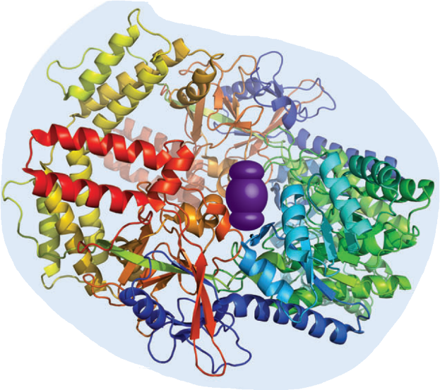
(or substrate) is an often small molecule that binds a certain protein with high affinity and specificity (see
Figure 1). The protein has often a defined three-dimensional conformation, that provides a binding pocket fully engulfing the ligand and, thereby, maximizing the binding contact. Hence, protein-ligand binding often shows selectivity,
e.g.
for the size, shape and electrostatic characteristica of the ligand (“lock-and-key” principle). One out of many impressive protein-type hosts is streptavidin that displays one of the highest affinities known for a small molecule (biotin) in aqueous
media (Ka = 3 ∙ 1013 M−1).
[6]
On account of its reliably strong and selective complex formation, the (strept)avidin-biotin pair has found a wide range of supramolecular, biochemical, and biotechnological applications.
[7-9]
Furthermore, if proteins consist of more than one subunit, the binding affinities of these subunits can be regulated
via
allosteric control
of an effector molecule. Allosteric processes are closely associated with ligand-induced conformational changes of a protein subunit that propagate towards coupled binding sites in other subunits of the same protein. Typical examples are the
classical homotropic oligomeric systems such as haemoglobin, where the binding of oxygen to one of the subunits is affected by its interactions with the other subunits. If one oxygen molecule binds, the other subunits have a higher affinity to bind
oxygen which is one example for a positive cooperative effect.
[11,12]
Practically, protein-ligand complexes are used for antibody-based biosensors and in ELISA assays due to their great reliability, high
binding affinity, and selectivity. However, protein based biosensors have a range of disadvantages: their low stability under physiological conditions, the limited range of detectable analytes and their high price.
[13]
Moreover, the internalization of antibodies and other proteins into living cells is tedious. Thus, real time analyte detection and reaction monitoring under physiological conditions faces complications with protein-based biosensors.
Artificial host systems
Compared to biological protein–based receptors, artificial hosts are composed of much simpler, often rigid aromatic building blocks and/or are highly symmetric macrocycles. They are therefore typically much less selective in guest binding than their natural counterparts. Nevertheless, the use of artificial host-guest complexes facilitates systematic investigations of non-covalent interactions and molecular recognition principles in general. [14] The first classes of artificial hosts that were prepared, the crown-ethers and cryptands, efficiently recognize inorganic and simple organic cations, e.g. ammonium ions via ion–dipole interactions. [15] Nowadays, there is a great variety of hosts available that bind a wide range of guests. To make the host-guest complex formation more likely, the number of interaction motifs between host and guest can be increased (multivalency effect) or the conformational degree of freedom of the host can be reduced (macrocyclic effect). This is known as the pre-organization principle. In general, the Gibbs free energy of host-guest formation is a subtle interplay of enthalpic and entropic contributions of interactions between host, guest, and solvent. [4]
Note: Supramolecular systems are inherently complex and may show unexpected behaviour such as aggregation phenomena or formation of higher, e.g. heteroternary, complexes. We strongly advice the SupraBank users to carefully report on the concentration (ranges) of host, guest or indicator (=competitive binding guest) such that unnoticed complications and their implications for the reported binding parameters can be identified at a later stage of data re-use.
References
- Ed.: B. Wang, E. V. Anslyn, Chemosensors: Principles, Strategies, and Applications, John Wiley & Sons, Inc., 2011.
- F. Biedermann, H.-J. Schneider, Chemical Reviews 2016, 116, 5216-5300.
- E. Fischer, Berichte der deutschen chemischen Gesellschaft 1894, 27, 2985-2993.
- Ed.: C. A. Shalley, Analytical Methods in Supramolecular Chemistry, 2nd ed., 2012.
- P. Bongrand, Reports on Progress in Physics 1999, 62, 921-968.
- P. C. Weber, J. J. Wendoloski, M. W. Pantoliano, F. R. Salemme, Journal of the American Chemical Society 1992, 114, 3197-3200.
- E. P. Diamandis, T. K. Christopoulos, Clinical Chemistry 1991, 37, 625-636.
- C. M. Dundas, D. Demonte, S. Park, Applied Microbiology and Biotechnology 2013, 97, 9343-9353.
- O. H. Laitinen, H. R. Nordlund, V. P. Hytönen, M. S. Kulomaa, Trends in Biotechnology 2007, 25, 269-277.
- R. N. Dsouza, A. Hennig, W. M. Nau, Chemistry - A European Journal 2012, 18, 3444-3459.
- D. Kern, E. R. P. Zuiderweg, Current Opinion in Structural Biology 2003, 13, 748-757.
- J. Monod, J. Wyman, J.-P. Changeux, Journal of Molecular Biology 1965, 12, 88-118.
- S. Sinn, F. Biedermann, Israel Journal of Chemistry 2018, 58, 357-412.
- W. Nau, A. I. Lazar, S. Joshi, Angewandte Chemie International Edition 2011, 50, 8472-8473.
- C. J. Pedersen, Journal of the American Chemical Society 1967, 89, 7017-7036.
Assay type
Many different techniques have been devised to examine and understand host-guest complexes and their binding properties. The various methods are categorized in different types of assays depending on the type of host-guest complex formed. The terminus guest is used in the following sections for either guest or ligand molecules (in the context of protein-ligand interaction) and the terminus host is used for host and receptor molecules.
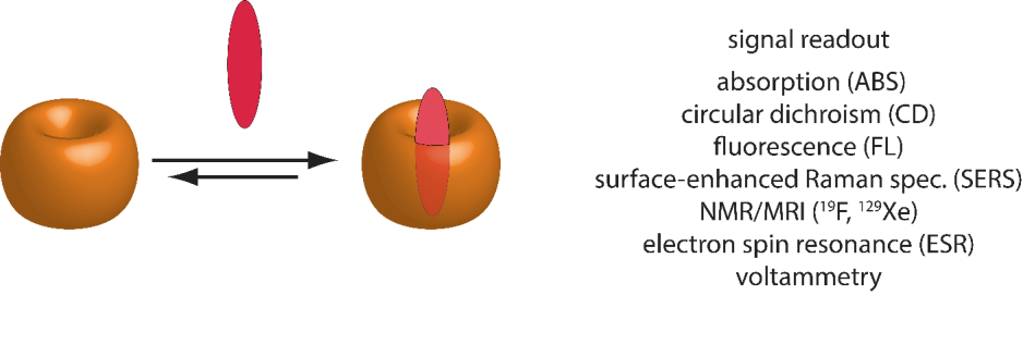
Direct-binding assay (DBA)
A direct binding assay (DBA) probes the interaction between a host and a guest molecule by its accompanying directly measurable output (e.g. heat increase/decrease or change in chemical shift) (see Figure 2). The binding affinity of the guest to the host is defined by the binding constant Ka. If the complexation of the guest leads e.g. to a change in the spectroscopic properties or a change in temperature (measurable by ITC) the binding affinity Ka can be determined through titration experiments.
Note: If salts are present in the solvent as e.g. in buffers, these ions may also bind as guests to the host and, therefore, affect the binding affinities of the host towards other guests. [1,2] At the SupraBank, salts in buffered solutions shall not count as competitive guests as long as the impact of the bound salt ions is not described explicitly in the original literature from which the data has been extracted. Generally, even if the host-guest complexation was studied in a buffer system, please use “DBA” regardless of the presence of possibly interfering salt ions.
Associative-binding assay (ABA)
The associative binding assay (ABA) is based on the binding of two guest molecules to one host molecule (see Figure 3). This is possible if the host has a sufficient large cavity to simultaneously bind two guest molecules having suitable sizes. The complexation can involve two different guest molecules, leading to a heteroternary complex as the one of CB[8] with MV and Trp-Gly-Gly.[SupraBank,8]
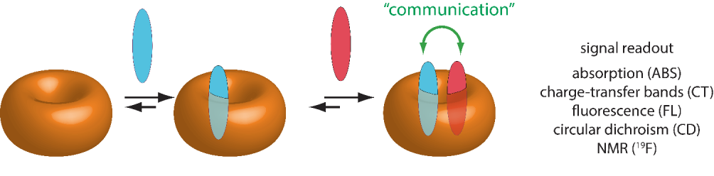
In heteroternary ABA, the host is usually first loaded with one of the guest molecules, and then in the next step the second guest is added. For systems such as the host cucurbit[8]uril, the binding of the second guest molecule takes place next to the preloaded molecule inside the cavity (stacking complex). The preloading of the host with an indicator gives a host-indicator complex with characteristic spectroscopic properties. The binding of the second guest can then be easily determined if the complexation of the second guest leads to a change in e.g. spectroscopic properties. For instance, addition of the second guest can cause a fluorescence quenching due to the close proximity of guest and indicator inside the host cavity.
Often, protein-ligand interactions are associative as the binding of a substrate happens only if a cofactor is present. Such associative binding are also cooperative (positive or negative). In the special case of allosteric control, the binding of a ligand to one subunit of the protein increases the affinity of neighbouring subunits to further ligands. These ligands can be either identical to the first ligand or different molecules. [3]
Competitive-binding assay (CBA)
The competitive-binding assay (CBA) is based on the competition between two different guest molecules for a host molecule. In the simplest case, the guest molecule with the higher binding affinity for the host displaces the guest molecule with the lower binding affinity, assuming that the concentration of both guests are similar (see Figure 4). However, as supramolecular binding phenomena are usually reversible and adhere to the mass law, a strongly binding guest can be also displaced from a host by a weaker binding guest if the latter is added in a large stoichiometric excess. CBA are mainly used to overcome signal monitoring difficulties, e.g. with spectroscopically silent host and guests, or, when the binding of the host and guest of interest is too strong under the selected experimental conditions, preventing the direct binding affinity determination by DBA or ABA.
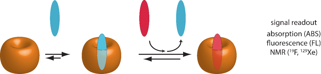
The most utilized CBA in supramolecular chemistry is the indicator displacement assay (IDA), which is commonly used for the determination of the binding affinity of a spectroscopically silent guest molecule to a spectroscopically silent host molecule. [6,7] In this way, the difficulty with monitoring spectroscopically silent host-guest complex formation can be solved elegantly by utilizing a spectroscopically active indicator dye as an auxiliary (guest B). The indicator should possess a sufficiently high affinity for the host and should show distinctly different photophysical properties (e.g. absorbance or absorbance wavelength, emission intensity or emission wavelength, or excited state lifetime) in its free and bound form. The competitive displacement of the host-bound indicator B upon addition of guest A leads to an increase in concentration of free indicator B, causing a characteristic signal change that is utilized for fitting the binding affinity of the spectroscopically silent host-guest complex. The reverse set-up, i.e. host-guest complex formation followed by the competitive displacement of the guest A through stepwise addition of indicator B is an alternative, recently disclosed method for determining host-guest binding affinities. It has been termed guest-displacement assay (GDA). [8] A software package thermoSimFit for planning of IDA and GDA experiments, and for fitting of the obtained experimental data can be obtained free of charge.
Besides optical spectroscopy, also NMR-based signal monitoring can be applied in CBA. This can be particularly useful if the indicator utilized has special properties, e.g. has atoms having chemical shifts far distinct from other potentially overlapping signals of the host and guest. NMR-monitored CBA with, for instance 1H or 19F NMR active indicators, is also useful if the guest, e.g. noble gases, do not show any useful NMR signals. Also, gases cannot be easily titrated to a solution and, hence, the gas molecules are preloaded to the host and, subsequently, replaced by another guest in order to monitor the reaction pathway. CBA is also often applied to NMR-based host-guest complex formation monitoring if the suspected host-guest affinity is unsuitably strong and thus out of the range that can be obtained by NMR-based DBA, e.g. Ka >> 103 M−1 for NMR experiments conducted at the mM concentration range.
Another common competitive binding assay is the competitive isothermal titration calorimetry (ITC) that is set-up if the guest A, the molecule of interest, has a binding affinity too high to be determined in a direct manner by ITC (i.e. Ka > 109 M-1). Therefore, the host is preloaded with another guest B, a competitor that has a binding affinity towards the host by a factor of ~ 103 M-1 lower than that of guest A. Then, this guest A is titrated to the mixture containing the host preloaded with guest B. The binding curve (titration curve) is flattened due to the additional free energy cost for competitor replacement, as the guest first has to replace the already prebound competitor before binding to the host. Through the software packages provided by the ITC manufacturers, the binding constant of guest A can be calculated from the experimental data either relatively to the binding constant of guest B or absolutely in the case that the binding constant of guest B is known. [4,5]
Note: In SupraBank, it can be specified for IDA-derived binding parameters at which concentration the host and indicator were utilized, and in which concentration range the guest was added. Likewise for GDA, the concentration of host and guest
can be reported, and the concentration range of the indicator that is added stepwise can be provided. Supramolecular systems are inherently complex and may show unexpected behaviour such as aggregation phenomena or formation of higher,
e.g.
heteroternary, complexes. Because a CBA system is inherently more complex than the binary mixture of host and guest used for DBA, we strongly advice the SupraBank users to carefully report on the concentration (ranges) of host, guest and indicator
(=competitive binding guest) such that unnoticed complications and their implications for the reported binding parameters can be identified at a later stage of data re-use.
Furthermore for NMR-based CBA, both the “reporting” nuclei and the chemical shift that was used as the observable can be specified in SupraBank.
References
- H. Tang, D. Fuentealba, Y. H. Ko, N. Selvapalam, K. Kim, C. Bohne, Journal of the American Chemical Society 2011, 133, 20623-20633.
- S. Zhang, L. Grimm, Z. Miskolczy, L. Biczók, F. Biedermann, W. M. Nau, Chemical Communications 2019, 55, 14131-14134.
- M. F. Perutz, 3-25. In: Eds.: K. Reinhart, Clinical Aspects of O2 Transport and Tissue Oxygenation, Springer-Verlag 1989.
- S. Moghaddam, C. Yang, M. Rekharsky, Y. H. Ko, K. Kim, Y. Inoue, M. K. Gilson, Journal of the American Chemical Society 2011, 133, 3570-3581;
- M. V. Rekharsky, T. Mori, C. Yang, Y. H. Ko, N. Selvapalam, H. Kim, D. Sobransingh, A. E. Kaifer, S. Liu, L. Isaacs, W. Chen, S. Moghaddam, M. K. Gilson, K. Kim, Y. Inoue, Proceedings of the National Academy of Sciences 2007, 104, 20737-20742.
- Ed.: P. D. C. Schalley, Analytical Methods in Supramolecular Chemistry , Wiley‐VCH Verlag 2006.
- S. L. Wiskur, H. Ait-Haddou, J. J. Lavigne, E. V. Anslyn, Accounts of Chemical Research 2001, 34, 963-972.
- L. M. Heitmann, A. B. Taylor, J. Hart, A. R. Urbach, Journal of American Chemical Society 2006, 128, 12574–12581.
- S. Sinn, J. Krämer, F. Biedermann, Chemical Communications 2020, 56, 6620-6623.
Techniques
Isothermal titration calorimetry (ITC)
Isothermal titration calorimetry (ITC) [1-4] is an often used method in supramolecular chemistry and protein science that measures the heat change occurring if two molecules interact with each other, i.e. heat release or heat uptake (see Figure 5). In supramolecular reactions, the heat is released or consumed due to redistribution and formation of non-covalent bonds and the re-organization of solvent molecules during the complexation process.
Note: Typically, ITC measurements are conducted in aqueous media, but can be also performed in some organic solvents. Both in supramolecular chemistry and protein-science, it has been frequently observed that even relatively small differences in the reaction media, i.e. aqueous solutions that differ in the salt concentration or potentially used co-solvents (as e.g. DMSO to solubilize the ligand), can have an pronounced impact on the obtained thermodynamic parameters, particularly on ΔH and TΔS. SupraBank offers therefore the option to accurately describe the media in detail as buffer or complex solution having additives in order to facilitate the comparison between results obtained by different operators.
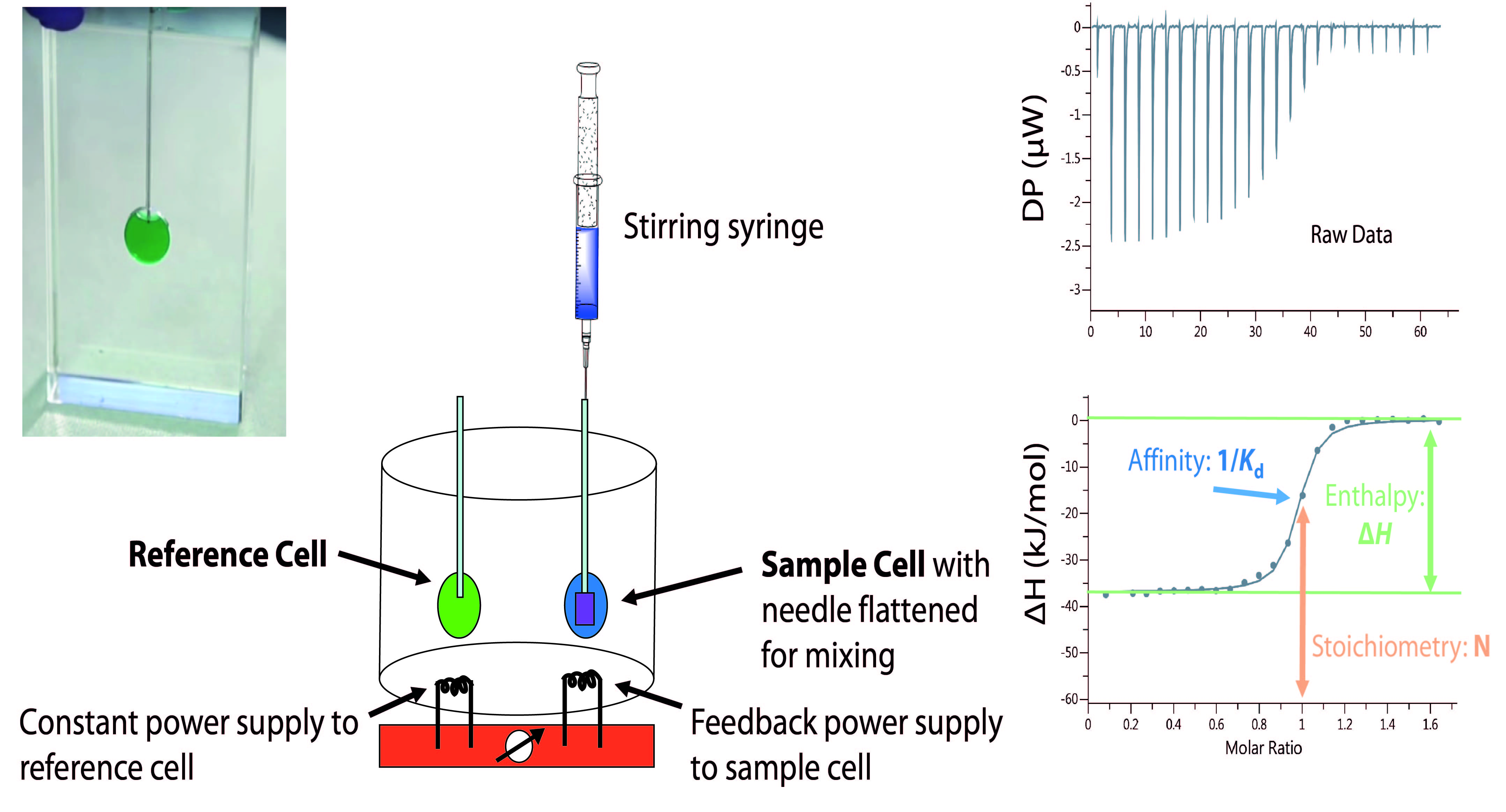
The calorimeter used in ITC contains two cells which typically have cell volumes between 1.5 ml and 2 ml, microcalorimeters have cell volumes around 200 µl. One cell is the sample cell, the other is the reference cell (see Figure 5). Each of the cells is seated in an insulated compartment typically regulated 5 K – 10 K above the environmental temperature to allow a cooling heat flow. The reference cell is continuously heated to the reference temperature. The temperature in the sample cell is automatically regulated by an electrical heater in order to minimize the temperature difference between the cells. The reference cell usually contains water while the sample cell contains an aqueous solution of one of the binding partners. A stirring syringe injects a solution of the other binding partner into the sample cell, typically in 0.5 µl to 4 µl aliquots until the concentration of this partner is two- to three-fold higher than the sample concentration. On injecting aliquots, the association of the binding partners produces a heat effect that raises or lowers the temperature in the sample cell. The deflection of temperature triggers the feedback regulator to adjust the electrical power needed to maintain identical temperatures in both cells. The change in the respective feedback current is the primary signal observed and corresponds to a heat pulse (heat production over time). This measurement parameter is called the differential power (DP) (see Figure 5). Each injection results in a heat pulse that is integrated with respect to time and normalized for concentration to generate a titration curve of the heat Q vs. molar ratio. The resulting isotherm is fitted by a binding model to generate the binding affinity (Kd = 1/Ka), stoichiometry (N) and enthalpy of interaction ΔH.
Note: As one binding partner is added in many aliquots from the syringe to the cell solution, the concentrations of both partners in the cell change. In the SupraBank, the option "varied" shall be chosen for the binding partner in the syringe. For the binding partner, which is in the cell from the beginning, only a mean concentration shall be stated. The limits of the varied concentation of the partner added by the syringe can be calculated in the following manner: the start concentration is 0 M-1 as there is not yet any aliquot added. The end concentration is the number of aliqouts times the volume of the aliquots times the concentration in the syringe solution divided by the volume of the solution in the cell. The volume of the solution in the cell at the end is the volume of the solution in the cell at the beginning and the volume added through the aliquots.
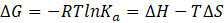
The knowledge of the complex stability constant Ka and the molar enthalpy ΔH enables the calculation of the Gibbs free energy ΔG and entropy ΔS according to
It has been widely accepted that the
C-value
(or sigmoidocity factor) with C=N*chost or guest in the cell*Ka
provides a good starting point to judge the reliability and error-range of the binding affinity
Ka
and the molar enthalpy ΔH
obtained by ITC under the particular experimental conditions chosen.
In general, an optimal C-value range of 5 to 500 is recommended for binding affinity determinations. Conversely, the most accurate ΔH
values are obtained when the ITC titration curve resembles a step-function. In our experience, C-values > 50 are preferred for accurate ΔH
determination, but a C-value of ~ 10 may be sufficient for obtaining reasonable ΔH
estimates. Reliable ΔS
values are therefore only obtained if both the ΔG
and ΔH
values are reasonably accurately determined. If ΔS
is determined from one set of ITC experiments, it is therefore recommended that the C-value lies in the range of 10-500.
Note: In order to allow for consideration of the C-value when comparing binding parameters listed in SupraBank, we recommend that the user provide the necessary information, i.e. concentration of the guest or host in the cell.
Note: In SupraBank, you can enter ΔH and the term -TΔS in kJ mol-1 or kcal mol-1 as well as ΔS in J mol-1 K-1 or cal mol-1 K-1. The corresponding values in the other unit or the term -TΔS and S are calculated automatically. However, only the value of ΔH and the term -TΔS in kJ mol-1 are saved to the SupraBank database. This means that the value for e.g. ΔS in cal mol-1 K-1 displayed in the interaction overview after saving can differ slightly from the original entered value due to rounding.
Information output:
- binding affinity (Ka)
- stoichiometry (N)
- thermodynamic data (ΔH, ΔG, ΔS)
- F. P. Schmidtchen, Isothermal Titration Calorimetry in Supramolecular Chemistry. In: Eds.: P. A. Gale, J. W. Steed Supramolecular Chemistry: From Molecules to Nanomaterials 2012, Wiley.
- S. Moghaddam, C. Yang, M. Rekharsky, Y. H. Ko, K. Kim, Y. Inoue, M. K. Gilson, Journal of American Chemical Society 2011, 133, 3570-3581.
- A. Saboury, Journal of Iranian Chemical Society 2006, 3, 1-21. (protein interaction)
- S. Leavitt, E. Freire, Current Opinion in Structural Biology 2001, 11, 560-566. (protein interaction)
- Short introduction to ITC by TA instruments.
- V. Frasca, Best practices for ITC to study binding interactions 2019.
ITC data acquisition example
This is an example for data acquisition from the outputs of an experiment conducted with the MircoCal PEAQ-ITC by Malvern Pananalytical.
ITC data acquisition
In Figure 5a, there is an example how to extract the parameters needed for the SupraBank from the outputs of an experiment conducted with the MircoCal PEAQ-ITC by Malvern Pananalytical.
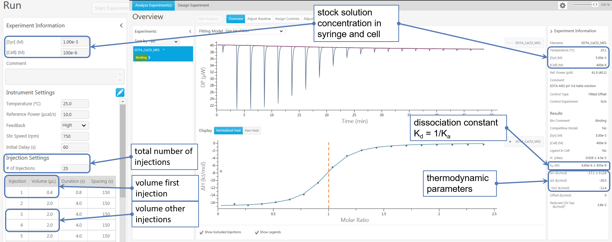
Note: In SupraBank, you can enter either directly the concentrations of the substances or the ITC parameters shown in Figure 5a. In the second case, Suprabank automatically calculates the substances' concentrations. SupraBank approximates concentrations of substances in the cell to be constant:

Of course, also these concentrations will change slightly as the volume in the cell increases by the injections of the syringe. For the substances in the syringe, the concentration range in the cell is calculated as follows. In the beginning, the concentration in the cell is zero as nothing has been added from the syringe:

During the injection from the syringe to the cell, the amount of substance remains constant:

with

Hence, the upper concentration of the substance injected in the cell is:
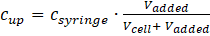
If some of the parameters are unknown, SupraBank makes approximations:
If the volume of the first injection Vinit is not given, SupraBank assumes that it is equal to the injection volume Vinjection of the further injections. Consequently, the assumed added volume and the upper concentration are probably slightly overestimated.
If the volume of injections Vinjection or the number of injections Ninjection is not given, SupraBank assumes that the complete syringe volume is added to the cell:
and, thus, calculates only an overestimate of the concentration range.
Nuclear magnetic resonance (NMR)
Nuclear magnetic resonance (NMR) spectroscopy is a method used to examine the electronic environment of single atoms and their interaction with their neighbor atoms. It enables the elucidation of the structure and molecular dynamics as well as of concentrations of a sample.
Nuclear magnetic resonance is based on the interplay of an external magnetic field with the magnetic moment of the atomic nucleus. The magnetic moments of atomic nuclei are directly correlated to their spin S and only nuclei with a spin S≠0 show a magnetic moment. In organic chemistry, preferrably nuclei with a nuclear spin S=1/2 are examined, i.e. 1H, 13C, 15N, and 31P. [5]
Theoretical Background of NMR [5-7]
Without an external magnetic field, all nuclear spin orientations for S=1/2 are energetically equal, but in the presence of an external magnetic field B0, the nucleic spins orientate either parallel (α) or antiparallel (β) to the external magnetic B0-field (see Figure 6). Due to the Boltzmann distribution, the parallel and, thus, lower energetic α-state is (slightly) higher populated than the β-state. This leads to a macroscopic magnetization in B0 (longitudinal), where all nuclear spins move in a precession along the magnetization. In order to generate a signal, a short pulse (short term magnetic field with high frequency) is induced causing a flip of the magnetization Mz along a certain phase. Figure 6 illustrates a 90 ° pulse causing a flip with the degree p along the y-axis. The magnetization Mx starts to rotate along the z-axis with the precession frequency ω, which is defined as ω = γ*Beff. The local magnetic field Beff is influenced by the local electron density.
As Beff is very similar in magnitude to B0, there is only a small difference between the ω of different nuclei. In a rotating coordinate system, the detector is moving with the frequency ω0 along the z-axis. Therefore, only the difference ω-ω0, the precession frequency Ω, can be registered by the detector. The precession frequency Ω is the oscillation frequency of the signal S(t), also known as free induction decay(FID),which can be translated into a spectrum with a signal at the frequency Ω via Fourier transformation.
The liquid NMR measurement of a molecule is carried out by dissolving the sample in a deuterated solvent (e.g. D2O) in an NMR tube. The tube is placed into a homogenous magnetic field inside the spectrometer and a high frequency pulse is induced, causing signals S(t), which are Fourier-transformed into a frequency spectrum of the sample.
The chemical shift δ of the spectra signal is given in parts per million (ppm) and is referenced to a standard, making δ independent from the used external magnetic field strength and spectrometer.
The chemical shift for protons is dependent on their chemical environment causing different shift ranges for different functional groups. The integration of the signal gives the relative number of protons corresponding to the signal. Taking the information from the chemical shift, relative signal integrals and potentially additional sources of information such as 13C NMR or 2D-NMR spectra into account, it is in most cases possible to elucidate the molecular structure of the unknown compound.
NMR in supramolecular chemistry [5-7]
NMR spectroscopy is often used in supramolecular chemistry to examine host-guest complexes because the nuclei of host or guest molecules usually experience a change in the electron density and local magnetic fields upon complex formation. The resulting change of chemical shifts and signal intensities can be observed by NMR spectroscopy.
Generally, host-guest complexes have certain equilibrium exchange rates r and, thus, each of the states, bound and free, has a certain lifetime τ. For some of the nuclei, the local magnetic field differs significantly between the bound and the free state due to changes in the electron density and, hence, there is chemical shift difference for these nuclei between the two states. This chemical shift difference gives the relevant NMR time scale. In general, only nuclei can be studied for which this chemical shift difference is clearly different from the equilibrium exchange rate v , from the rate of complex formation. [8]
If the equilibrium reaction rate v is large compared to the chemical shift difference between the two stabilities due to fast (de)complexation, the reaction is fast on NMR time scale and the two signals merge to one averaged signal. This is often the case in NMR titration of supramolecular complexes. Therefore, one compound is added stepwise to the other and the change of the chemical shift is monitored over the concentration variation. Then, the binding affinity Ka can be determined by fitting the curve of the obtained data points (Δδ vs. concentration). [15,16]
If the equilibrium exchange rate is slow on the NMR time scale (so the nuclei change their environment slowly due to slow complexation), the signals of the nuclei in the free state and in the host-guest complex appear at their individual chemical shifts. The signal integral gives a measure for the concentrations of both states. In this case, a Job plot or the best fit approach yield the stoichiometry of the complex.
Note: If this or any other method has been utilized to confirm the presumed host-guest binding stoichiometry, please indicate this in the “comments field” provided in SupraBank.
Furthermore, NMR spectroscopy can uncover hidden aggregation phenomena of supramolecular systems, which may be relatively common in the concentration range (~ mM) needed for NMR analysis. Typical indications are line-broadening. Powerful NMR
methods such as diffusion-ordered spectroscopy DOSY provide additional indications for the formation of aggregates or higher complexes. If experimental data is available indicating aggregated superstructures in solution at the concentration range
probed, please indicate this in the comments field provided in SupraBank.
Information output:
- binding affinity (Ka)
- stoichiometry (N)
- concentration (c)
- complex conformation
- Z. R. Laughrey, C. L. D. Gibb, T. Senechal, B. C. Gibb, Chemistry – A European Journal 2003, 9, 130-139.
- R.-C. Brachvogel, H. Maid, M. von Delius, International Journal of Molecular Science 2015, 16, 20641–20656.
Photophysics – introduction
The principals of light absorption and emission of molecules can be well explained using the Jablonski diagram [9] (for a simplified version see Figure 7), which illustrates the different transitions between electronic states (S = singlet, T = triplet) of a molecule after the absorption of a photon with a suitable energy. The irradiation of a molecule with light can lead to the absorption of a photon, which results in the transition of the molecule from its ground state ( S0, ν0) to an exited state (e.g. S1) with a higher vibrational level (e.g. ν4). From here, the molecule can quickly relax to its vibrational ground state of the excited state (S1, ν0) via a non-radiative relaxation. From there, the molecule can go back to the molecule's ground state S0 by the radiative process resulting in a fluorescence emission or by non-radiative relaxation associated with heat release. Since a part of the energy of the absorbed photon is converted into heat through non-radiative relaxation to the vibrational ground state of the excited state (S1,ν0) prior to radiative relaxation to the ground state S0, the emission band is typically (few examples such as azulene exist) of lower energy (Stokes shift) compared to the absorbance band, but both can intersect.
UV/Vis Absorption spectroscopy (ABS)
Absorption spectroscopy is a widely used technique in analytical chemistry which uses the wavelength dependent absorption characteristics of materials to identify and quantify specific substances.
The absorption of a photon leads to the transition of an electron from the ground state (S0) to an excited state (Sx with x>0), see Jablonski diagram. The wavelength of the absorbed photon is hereby dependent on the energy gap between Sx and S0. If the energy gap is small, light having a small energy and, thus, a long wavelength is absorbed.
Employing Lambert-Beer’s law, the absorbance A of a molecule can be used to determine its concentration in the measured solution as the law states that the absorbance A is directly proportional to the concentration c of the absorbing species. [7,11] The absorbance A is a dimensionless quantity and is the degree of the light intensity reduction after crossing a certain matter e.g. the sample cell:
with ε: molar extinction coefficient, c: concentration of species, and d: path length of the light in the sample cell.
The absorbance is often measured at a double beam spectrometer (see Figure 8), where a continuous light source (e.g. xenon lamp) irradiates light in a defined range, e.g. 200 nm - 1000 nm. The light beam passes the monochromator, selecting one wavelength, and is then split into two beams. One beam passes the sample and the other passes the reference (e.g. the neat solvent). The beams are collected in the detector, compared by the multiplier and, then, transferred into data (spectrum).
Absorption spectroscopy is commonly used to examine the binding affinities of two molecules to each other (e.g. host-guest complexes), by measuring the absorbance of the formed complex during the titration of one species to the other. Here, often the host is added stepwise to a guest solution and the absorbance is measured after each addition. The binding affinity Ka can then be determined by fitting the curve of the obtained data points (absorbance vs. concentration of the host) (see Figure 9). [12]
Information output:
- binding affinity (Ka)
- stoichiometry (N) via Job Plot or best fit approach
- concentration c of the complex
- A. R. Bernardo, J. F. Stoddart, A. E. Kaifer, Journal of American Chemical Society 1992, 114, 10624-10631.
- Z.-Z. Gao, J.-L. Kan, L.-X. Chen, D. Bai, H.-Y. Wang, Z. Tao, X. Xiao, ACS Omega 2017, 2, 5633-5640.
Fluorescence spectroscopy (FL)
Fluorescence spectroscopy [13] is a common method in analytical chemistry for quantitative and qualitative analysis of molecules.
The excitation of a molecule is stimulated by the absorption of a photon, which leads to the transition from the ground state (S0) to an excited state (SN with N > 0) (see Jablonski diagram)) On account of ultra fast processes such as internal conversation (IC) vibrational and cooling the system relaxes typically quickly into the first electronically excited state (fluorophors: S1, phosphors: T1) featuring the lowest vibrational state (v0) (Kasha’s rule). The radiative decay without alteration of the spin is called fluorescence, commonly the transition from S1 -> S0. The radiative process comprising a spin alternation is called phosphorescence, typically T1 -> S0.
The setup of a fluorescence spectrometer is shown in Figure 10. The irradiated light which is thinned out by a slit and passes to the monochromator, which selects a certain wavelength. The transmitted light passes the sample, resulting in an excitation, followed by fluorescence emission of the excited molecules. The fluorescence light is often measured in a 90 ° angle to the excitation light, to avoid interferences. The emitted light is collected by the detector and transferred into a spectrum.
The emission intensity correlates typically linear with the concentration of the fluorescent molecule if inner filter effects can be excluded. [13] Thus, fluorescence spectroscopy can be used to probe the concentration of an emitting species, e.g. the free indicator or the indicator-host complex. The binding constant can be determined by detecting the emission change for a variety of concentration ratios and fitting the curve of the obtained data points. [16]
In host:guest chemistry, fluorescence spectroscopy is commonly used to examine the binding affinities and rate constants of two molecules to each other (e.g. host-guest complexes) by measuring the fluorescence emission during the titration of one species to the other. The complex formation causes a change in the environment of host and guest molecules and can result in a:
- Decrease in the fluorescence intensity
- Increase in the fluorescence intensity
- Appearance of a new emission band
Information output:
- binding affinity (Ka)
- stoichiometry (N) via Job plot or best fit approach
- concentration c of complex
- binding kinetics (using stopped-flow technique)
- lifetime (applying specific calculation or instrumentation)
- quantum yield (using laser setups)
- Z. Miskolczy, L. Biczók, G. Lendvay, Physical Chemistry Chemical Physics 2018, 20, 15986-15994.
- F. Biedermann, D. Hathazi, W. M. Nau, Chemical Communications 2015, 51, 4977-4980.
Circular dichroism spectroscopy (CD)
Circular Dichroism (CD) spectroscopy measures the differential absorption of left- and right-circularly polarized light by a chiral sample. It occurs in correspondence with electronic and magnetic transition dipole moments and represents the chiroptical counterpart of the more common UV-Vis absorption spectroscopy. Hence, it is sensitive to the absolute configuration and total molecular structure of the sample. This means while the two enantiomers of a chiral substance will have identical UV-Vis, IR and Raman spectra, they will have distinguishable, mirror-image looking CD spectra. [17,18]
If A is the absorption of the sample from non-polarized light and AL and AR are the absorptions of left and right circularly polarized light (L- and R-CPL), the absorption CD is defined as:
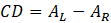
This quantity is usually measured in mdeg units.
A standard CD spectrometer is similar in design to a normal spectrophotometer with a few differences (compare Figure 11 ). The incident light coming from the source (S) is passed through the monochromator (M) followed by a photoelastic modulator (PEM), which produces the left and right circularly polarized light (L- and R CPL). When circularly polarized light (CPL) passes through a sample possessing chirality, the decreases in amplitude of L- and R-CPL are different. This difference is the CD of the measured sample. The transmitted light is then amplified and the two signals are recombined (through a lock-in amplifier) to output the true CD signal collected by the photomultiplier (PMT).
CD spectroscopy is especially useful in protein science for analysing the secondary structure or conformation of macromolecules or proteins as secondary structure is sensitive to its environment, temperature or pH. However, most bioactive small molecules such as amino acids are non-chromophoric or absorb below 280 nm of the electromagnetic spectrum. Besides, small molecules are typically conformationally flexible, giving an averaged CD signal. Thus, CD spectroscopy is of limited use in detecting or characterizing metabolites, hormones, or peptides.
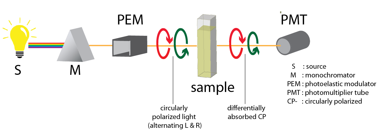
In recent years, molecular recognition-based approaches were introduced for chirality sensing of chromophoric small molecules by CD spectroscopy. Therefore, supramolecular optical sensors were developed which interact with the chiral analyte via covalent or non-covalent interactions to give rise to spectroscopic responses in the visible region (see Figure 12 ). [19-21] In the simplest case, the binding of a chiral analyte to an achiral chromophoric host can give rise to induced CD (ICD) signals in the near-UV or visible region of the latter. The induction of chirality can occur either by an electronic coupling between the chromophoric host and the chiral guest in case of rigid host molecules or by the deformation of the host into a chiral conformation upon guest binding in case of flexible host molecules. [22] In favourable cases, analyte-specific “ICD fingerprints” occur, which can be utilised for analyte identification and differentiation. [23]
Information output:
- Chirality
- Optical purity
- K. W. Bentley, Y. G. Nam, J. M. Murphy, C. Wolf, Journal of American Chemical Society 2013, 135, 18052-18055.
- G. A. Hembury, V. V. Borovkov, Y. Inoue, Chemical Reviews 2008, 108, 1-73.
Surface enhanced Raman scattering (SERS)
In Raman spectroscopy, spectra of the scattered instead of the absorbed or emitted light are detected. [25] As IR spectroscopy, Raman spectroscopy probes vibrational degrees of freedom. If light is scattered by a material, most photons are scattered elastically. This means that the photons have the same energy as the incident photons, but a different direction. This Rayleigh scattering usually has an intensity of about 0.1 % to 0.01 % of that of the radiation source being mostly a laser with visible or Near Infrared (NIR) radiation. An even smaller fraction of the photons, about one in a million, is scattered inelastically. The energy of the scattered photons is either photons is either higher (Anti Stokes) or lower (Stokes) than that of the incident photons.
In general, the intensity of Raman scattering is very small compared to the incident light as so few photons are scattered inelastically. If single molecules or analytes in very low concentrations shall be studied, an enhancement is often needed. One method is the surface-enhanced Raman Spectroscopy (SERS). If molecules are adsorbed on rough metal (e.g. silver or gold) surfaces or on metal nanostructures, Raman scattering is strongly enhanced by a factor of up to 1010 or 1011. [24] Thus, this immense enhancement enables the detection of even single molecules. Silver and gold are typical metals for SERS experiments as their plasmon resonance frequencies fall within the visible and NIR range used for Raman scattering. However, the metal particles or surfaces need to have the right size or structure in order to create the so-called hot spots having high local field intensities. Unfortunately, it is difficult to create stable aggregates of a given size that do not aggregate further, but supramolecular hydrogels are tested for stabilisation. [38]
For supramolecular chemistry, SERS measurements offer the possibility to study the orientations of molecules in host-guest complexes and to the surface. Basically, the modes present in the SERS spectrum depend on the exact orientation of the molecules due to the connected symmetry changes as Raman scattering is based on a change in polarizability. [39] Additionally, a qualitative assessment of analytes is possible by carrying out a principal component analysis of the spectral changes upon analyte variation and the binding constant Ka can be determined. [26] Furthermore, it is possible to differentiate different guests by the application of pattern recognition algorithms. [26]
Information output:
- Detection of single molecules or very low concentrations
- Orientation of adsorbed molecules
- T. R. Canrinus, W. W. Y. Lee, B. L. Feringa, S. E. J. Bell, W. R. Browne, Langmuir 2017, 33, 8805-8812.
- B. de Nijs, M. Kamp, I. Szabo, S. J. Barrow, F. Benz, G. Wu, C. Carnegie, R. Chikkaraddy, W. Wang, W. M. Deacon, E. Rosta, J. J. Baumberg, O. A. Scherman, Faraday Discussions 2017, 205, 505-515.
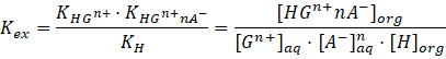
Extraction (EXT)
In extractions, an analyte is transfered from one phase to another immiscible phase by complexation with an extractant.
[35]
This can be used in cleaning, recycling, or analytical applications as well as in the study of the underlying processes. Typically, the analytes are ionic.
Hereinafter, the extraction process will be described in a simplified form based on the overall extraction equilibrium for the example of a salt GA. In the beginning, the free host H, a neutral macrocyclic extractant, is solved in the organic phase
whereas the guest (analyte) Gn+ and its counterion A-
are in the aqueous phase. Next, both phases are mixed well. An equilibrium of the free host between both phases is established, described by an equilibrium constant
KH. The free host in the aqueous phase forms a complex with the guest Gn+. This equilibrium is characterized by the binding constant
KHGn+
. The loaded host is transported to the organic phase with the equilibrium constant
KHGn+nA-
. Herein, this extracted complex needs a pronounced lipophilicity to achieve a good extraction. The equilibrium constant of the overall extraction
Kex
is:
Experimentally, the distribution ratio Danalyte can be measured e.g. using the radiotracer micro-extraction technique with radiolabeled anaylytes. [36]
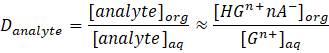
Combining this with the equation for the extraction constant Kex gives:

In a second step
via
back extraction, the separated analyte can be obtained and the extractant can be recovered.
Mostly, the extraction equilibrium is much more complicated due to other interactions in the two phases and several different species involved.
[37]
For instance, solvation or desolvation of both host and guest may influence significantly the phase transfer. Both enthalpic and entroptic effects are common. Additionally, processes as host aggregation or oligomerization may occur. Hence, the
evaluation is often based on mathematical models including nonlinear regression methods.
One of the most important values obtained by extraction experiments is the distribution ratio D, also called partition coefficient P. For instance, the decadic logarithm log POW
describes the distribution of a substance between water and octanol and, thus, serves as a measure for hydrophobicity. This coefficient is of critical importance in the assessment of drugs.
Information output:
- binding affinity (Ka)
- stoichiometry (N)
- selectivity
- speciation
- phase transfer behavior
- partition coefficient P (distribution ratio D)
Potentiometry (POT)
In potentiometry, the activity of an analyte in aqueous solution is measured by a change in the potential difference E, i.e. the voltage between a working electrode and a reference electrode. [27] Mostly, ion-selective electrodes (ISE), also known as specific ion electrodes (SIE), are used. The potential difference is theoretically dependent on the logarithm of the ionic activity according to the Nernst equation: [28]
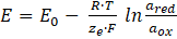
E is the potential at the temperature T, E0 is the standard potential, R is the universal gas constant, T is the temperature in Kelvin, ze is the number of electrons transferred in the reaction, F is the Faraday constant, ared is the chemical activity of the reduced analyte species, and aox is the chemical activity of the oxidized analyte species. Hence, this can be approximated by
In principle, electrodes can measure the potentials of both positive and negative ions and they are mostly unaffected by the sample color or turbidity. Electrodes showing (an)ionic selectivity often have an ion-exchange resin consisting of a specific ion-exchange agent, an ionophore, in an organic polymer membrane. The usage of specific resins allows the preparation of selective electrodes for different ions. However, such electrodes tend to have low chemical and physical durability compared to electrodes with glass or crystalline membranes. An example is the potassium selective electrode being based on valinomycin as ion-exchange agent. Valinomycin allows selectively the transport of potassium ions from the aqueous sample phase into the PVC-membrane and, thus, the potential of the working electrode changes. Hence, the fundamental chemical process is a guest – induced selective change in the charge separation at the interface between the membrane and the aqueous sample solution. This interface possesses unique properties, which are very different from the properties of the bulk phases. There, intermolecular recognition occurs between the analyte and the ionophore with extremely high selectivity and sensitivity.
Additionally, there are examples of detection of uncharged analytes. [29] Having added macromolecular hosts as calixpyrroles or corroles in a membrane resin, neutral species as phenol derivates were detectable. Also, it was possible to detect unprotonated aniline derivates in resins based on special calix[4]arenes or calix[4]resorcinarenes.
Information output:
- concentration c of the analyte
Examples:
Electronic paramagnetic resonance (EPR)
A method for the study of materials or molecules having unpaired electrons is the electron paramagnetic resonance (EPR) spectroscopy, also called electron spin resonance (ESR) spectroscopy. [30-32] In EPR as well as NMR, magnetic spins are excited and, thus, there are certain analogies. In EPR, electrons spins, resulting from unpaired electrons, are excited instead of atomic nuclei spins and, hence, a smaller external magnetic field is applied. Mostly, EPR measurements use microwave radiation in the 9 – 10 GHz region and external magnetic fields corresponding to about 0.35 T. [33] Typically, the radiation frequency is kept constant and the external magnetic field is varied in order to obtain a spectrum being called continuous wave EPR spectrum. Thus, the unpaired electrons, i.e. the paramagnetic centers, are exposed to microwaves of a fixed frequency. By increasing the external magnetic field, the energy difference between the electronic magnetic spin states m = ½ and m = −½ grows. If this difference matches the energy of the microwaves, the unpaired electron can change to the other spin state. Thus, there is a net absorption of energy. This absorption can be recorded. Often, the first derivative of the absorption spectrum is measured instead. Therefore, field modulation by a small additional oscillating magnetic field is applied to the external magnetic field at a typical frequency of 100 kHz. By using phase sensitive detection, only signals with the same modulation (100 kHz) are detected. Recording the peak to peak amplitude, the first derivative of the absorption is measured. This results in higher signal to noise ratios. Different to these continuous wave EPR spectra, spectra resulting from pulsed experiments are presented as absorption profiles.
EPR spectroscopy is particularly useful for studying metal complexes or organic radicals being used possibly as spin probes. Interactions of the unpaired electron with its environment influence the shape of an EPR spectral line. [33] The magnetic moment of a nucleus with a non-zero nuclear spin as e.g. H1 will affect the unpaired electrons. This leads to the phenomenon of hyperfine coupling, splitting the EPR resonance signal into doublets, triplets, and so forth. [32] For instance, the signal pattern can change significantly if an organic radical or metal ion is complexed in a supramolecular host. [34] If the exchange between the free and included radical are slow with respect to the EPR time scale (compare to NMR time scale), superposed spectra are observed. Then, the binding constant Ka can be determined by varying the host concentration and monitoring spectral changes. Furthermore, line shapes can yield information about, for example, rates of chemical reactions. [31]
Information output:
- binding affinity (Ka)
- concentration c of the analyte
- reaction rate r
References
- M. W. Freyer, E. A. Lewis, Methods in Cell Biology 2008,84, 79-113.
- J. E. Ladbury, Biotechniques 2004, 37, 885-887.
- A. A. Saboury, Journal of the Iranian Chemical Society 2006, 3, 1-21.
- W. B. Turnbull, A. H. Daranas, Journal of the American Chemical Society 2003, 125, 14859-14866.
- M. G. H. Kessler, M. Gehrke, C. Griesinger, Angewandte Chemie 1988, 100, 507-554.
- M. Holz, B. Knüttel, Physikalische Blätter 1982, 38, 368-374.
- J. de Paula, P. W. Atkins, Physical Chemistry, 11th Edition, Oxford University Press, 2017.
- R. G. Bryant, Journal of Chemical Education 1983, 60, 933.
- D. Frackowiak, Journal of Photochemistry and Photobiology B: Biology 1988, 2, 399.
- G. N. Lewis, M. Kasha, Journal of the American Chemical Society 1944, 66, 2100-2116.
- P. Wormell, A. Rodger, Absorbance Spectroscopy: Overview. In: Ed.: G. C. K. Roberts, Encyclopedia of Biophysics, Springer-Verlag, 2013.
- A. R. Bernardo, J. F. Stoddart, A. E. Kaifer, Journal of the American Chemical Society 1992, 114, 10624-10631.
- J. R. Lakowicz, Principles of Fluorescence Spectroscopy, 3rd edition, Springer, 2006.
- M. Kasha, Discussions of the Faraday Society 1950, 9, 14-19.
- Y. Cohen, L. Avram, T. Evan-Salem, S. Slovak, N. Shemesh, L. Frish, 197-285. In: Ed.: P. D. C. Schalley, Analytical Methods in Supramolecular Chemistry , Wiley‐VCH Verlag 2006.
- K. Hirose, Journal of Inclusion Phenomena 2001, 39, 193-209.
- N. Berova, L. Di Bari, G. Pescitelli, Chemical Society Reviews 2007, 36, 914-931.
- T. Smidlehner, I. Piantanida, G. Pescitelli, Beilstein Journal of Organic Chemistry 2018, 14, 84-105.
- K. W. Bentley, Y. G. Nam, J. M. Murphy, C. Wolf, Journal of American Chemical Society 2013, 135, 18052-18055.
- G. A. Hembury, V. V. Borovkov, Y. Inoue, Chemical Reviews 2008, 108, 1-73.
- L. You, J. S. Berman, E. V. Anslyn, Nature Chemistry 2011, 3, 943-948.
- A. Prabodh, D. Bauer, S. Kubik, P. Rebmann, F.-G. Klärner, T. Schrader, L. Delarue Bizzini, M. Mayor, F. Biedermann, Chemical Communcations 2020, 56, 4652-4655.
- F. Biedermann, W. M. Nau, Angewandte Chemie International Edition 2014, 53, 5694-5699.
- E. J. Blackie, E. C. Le Ru, P. G. Etchegoin, 2009 Journal of American Chemical Society 2009, 131, 14466–14472.
- Ed.: B. Schrader, Infrared and Raman Spectroscopy: Methods and Applications, Wiley VCH, 1995.
- B. de Nijs, M. Kamp, I. Szabo, S. J. Barrow, F. Benz, G. Wu, C. Carnegie, R. Chikkaraddy, W. Wang, W. M. Deacon, E. Rosta, J. J. Baumberg, O. A. Scherman, Faraday Discussions 2017, 205, 505-515.
- A. J. Bard, L. Faulkner, Electrochemical Methods: Fundamentals and Applications, 2nd edition Wiley, 2000.
- Eds.: M. V. Orna, J. Stock, Electrochemistry, past and present American Chemical Society, 1989.
- J. Radecki, H. Radecka, Potentiometry for Study of supramolecular recognition prodesses between uncharged molecules. In: Ed. G. Radis-Baptista, An Integrated View of the Molecular Recognition and Toxinology IntechOpen, 2013.
- E. Zavoisky , Fizicheskiĭ Zhurnal , 1945, 9 , 211–245.
- I. N. Levine, Molecular Spectroscopy Wiley & Sons, 1975, 380.
- J. E. Wertz, J. R. Bolton , Electron spin resonance: Elementary theory and practical applications Chapman and Hall, 1986.
- Eds.: D. Goldfarb, S. Stoll, EPR Spectroscopy: Fundamentals and Methods Wiley-VCU, 2018.
- S. Combes, K. T. Tran, M. M. Ayhan, H. Karoui, A. Rockenbauer, A. Tonetto, V. Monnier, L. Charles, R. Rosas, S. Viel, D. Siri, P. Tordo, S. Clair, R. Wand, D. Bardelang, O. Ouari, Journal of American Chemical Society, 2019, 141 , 5897-5907.
- H. Stephan, M. Kubeil, K. Gloe, K. Gloe, Extraction methods. In: In: Ed.: P. D. C. Schalley, Analytical Methods in Supramolecular Chemistry , Wiley‐VCH Verlag 2006.
- K. Gloe, P. Mühl, Isotopes in Environmental and Health Studies 1983, 19, 257-260.
- H. J. Schneider, A. Yatsimirsky, Principles and Methods in Supramolecular Chemistry, John Wiley & Sons, 2000 .
- T. R. Canrinus, W. W. Y. Lee, B. L. Feringa, S. E. J. Bell, W. R. Browne, Langmuir 2017, 33, 8805-8812.
- A. G. Brolo, Z. Jiang, D. E. Irish, Journal of Electroanalytical Chemistry 2003 547, 163–172.
Thermodynamics and Kinetics
Often, thermodynamic and kinetic parameters are described by equation systems, which cannot be solved analytically. In this case, numerical fitting and simulations can be used for the determination of e.g. the binding affinity or rate constants. Among others, the following two software packages were developed for this purpose:
-
thermoSimFit: a tool to simulate and fit binding isotherms and affinities
Download here: latest release.
Cite: S. Sinn, J. Krämer, F. Biedermann, Chemical Communications 2020, 56, 6620-6623.
Contribute: Mathematica software package ASDSE thermoSimFit. -
kineticSimFit: a tool for fitting kinetic data
Download here: latest release.
Cite: A. Prabodh, S. Sinn, L. Grimm, Z. Miskolczy, M. Megyesi, L. Biczok, S. Bräse, F. Biedermann, Chemical Communications 2020 56, 12327-12330.
Contribute: Mathematica software package ASDSE kineticSimFit.
Thermodynamics: binding affinity
Binding constant
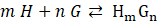
The binding constant Ka is a special case of the equilibrium constant K and describes the association of a host H (or receptor) and a guest G (or ligand).[1] The terms binding affinity, binding constant, and association constant are equivalent. The binding constant is inverse to the dissociation constant Kd, which characterizes the unbinding reaction of host H and guest G. The general binding constant Ka is described with
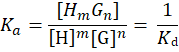
If m = n = 1, it is an 1:1 equilibrium of one guest forming a complex with one host:
with host concentration [H] in equilibrium, guest concentration [G] in equilibrium, host-guest complex concentration [HG] in equilibrium, initial host concentration [H]0, initial guest concentration [G]0, binding constant KaHG for the association of the host-guest complex, and dissociation constant KdHG for the dissociation of the host-guest complex.
The thermodynamic binding constant Ka is related to the kinetics of the particular system at equilibrium by:
This means that, in equilibrium, the forward (on) rate with which host and guest bind is equal to the backward rate with which the host-guest complex unbinds. Hence, the equilibrium concentrations are settled and the binding constant is given by the ratio of the forward (on) rate constant kin (M-1 s-1) and the backward (off) rate kout (s-1).
Additionally, the van’t Hoff equation relates the binding constant and its temperature dependence to thermodynamic parameters as enthalpy ΔH or the Gibbs free energy ΔG (also called free enthalpy):
with universal gas constant R, temperature T in K, and equilibrium constant K eq.
Unit and stoichiometry
Strictly speaking, equilibrium constants and, thus, binding constants, are defined based on relative activities and are therefore unitless. For solutions, mostly absolute concentrations instead of relative activities are considered and, accordingly,
the association constants based on concentration have units as M-x.
Table 1
gives an overview about common host-guest complex stoichiometry and the corresponding units.
Tab. 1: Examples of host-guest complex stoichiometries
| H:G ratio | Ka equation | unit | Example |
|---|---|---|---|
| 1:1 |
|
M-1 | direct-binding assay: e.g. cucurbit[7]uril (CB[7]) as host and phenylalanine as guest. [Suprabank] |
| 1:2 |
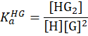
|
M-2 | direct-binding assay: two guests bind concertedly to one host, e.g. two N-terminal aromatic peptides as Trp-Gly-Gly in CB[8]. [Suprabank] |
| 2:1 |
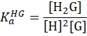
|
M-2 | direct-binding assay: one guest binds concurrently two hosts, e.g. the encapsulation of DABP by two CB[7] cavities. [Suprabank] |
| 3:1 |
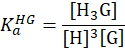
|
M-3 | direct-binding assay: three guest molecules bind concertedly to one host molecule, like the encapsulation of styrylcoumarin into three CB[7] molecules. [Suprabank] |
A popular method to determine the stoichiometry,
i.e.
the H:G ratio, is the
Job plot
or Job’s method.
[2]
The idea behind is really simple: if the sum of the total concentrations of host and guest is constant ([H]0
+ [G]0
= constant), the concentration of the complex HmGn
is at maximum when the concentration ratio [H]/[G] is equal to the H:G ratio (m/n). Practically, the host and guest concentrations are varied such that the sum of the total concentrations of host and guest is constant. Then, for instance, the
UV-Vis absorbance
or the
NMR chemical shift
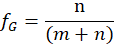
is detected giving a measure for the complex concentration. Finally, this signal read-out is plotted against the
mole fraction fG
of the guest with:
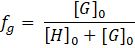
The maximum of the curve is at the mole fraction fG
The following Figure 13 shows a UV-Vis absorbance Job plot with an 1:1 stoichiometry of host and guest.

However, recent analysis [3] suggest to use Job plot only to verify a 1:1 complex as it is unreliable for other stoichiometries. A best fit approach with different binding models was found to be a better way for the stoichiometry determination. Among others, the software package thermoSimFit offers this best fit approach.
Note: If this or any other method has been utilized to confirm the presumed host-guest binding stoichiometry, please indicate this in the comments field provided in SupraBank.
Binding energy
The binding energy is the minimum energy required to disassemble a system of particles or molecules into separate parts. A measure for this energy is the Gibbs free energy calculated via the binding constant (see above). A good overview is given by Biedermann and Schneider.
[4]
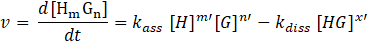
Kinetics: reaction rate
The reaction rate
v
is the speed at which molecules undergo reactions.
[4]
The reaction rate
v
of a host-guest complexation
is defined as
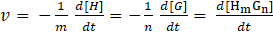
The reaction rate of the complex association obeys a rate law of the general form: [5]
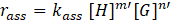
Herein, kass
is the rate constant and the exponents m’ and n’ are called partial orders of reaction and they are not necessarily equal to the stoichiometric coefficients m and n. Instead, they depend on the reaction mechanism and the underlining elementary steps.
Hence, the detailed study of the kinetics offers a way to elucidate the molecular reaction pathway.
The rate of dissociation is analogously
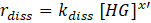
Hence, the reaction rate is:
Such rate laws for reversible reactions as host-guest complexation can typically only be solved numerically by software packages such as kineticSimFit. In order to find an analytical solution especially for systems involving more than two partners (competitive assays), physical meaningful approximations are necessary. [6-8]
Pseudo-first order
A common way to simplify a reversible bimolecular reaction is the so-called pesudo-first order approach, in which a second order system can be approximated as a (pseudo)first-order sytem. One reaction partner A, being either guest or host, is added in a huge excess of the other reaction partner B, being either host or guest. Thus, the concentration of B is approximately constant. In this case, nearly only
association occurs and the reaction can be observed under pseudo first-order conditions as
e.g.
for the reaction
 :
:
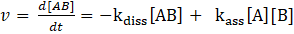
with
 and
and
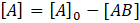 . This gives:
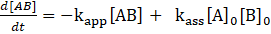
with
 . Thus:
As the pseudo first-order conditions accelerate the overall rate of reaction, mostly spectroscopic methods are used in such studies. However, it was shown that ITC titration experiments give similar exponential injection signals even under stoichiometric conditions and, thus, can be used for a analogous pseudo-first order determination of the rate constants. [9] For instance, the software package kineticSimFit can be used for such analyses.
Rate constant and activation energy
The rate constant k depends on the temperature as is described by the Arrhenius equation: [10]

with universal gas constant R, temperature T in Kelvin, the (possibly temperature dependant) pre-exponential factor A, and the activation energy Ea
of the reaction.
The activation energy describes the energy changes during the course of the on-going reaction or association. Thus, it describes the transition state. Molecules have to overcome an energetic barrier in order to react, associate or dissociate. This
energy needed is supplied by the thermal energy of the molecules, which differs from molecule to molecule as described by the Maxwell-Boltzmann distribution. The smaller the necessary activation energy, the more molecules have enough thermal energy
to react or associate. A deeper understanding of the physical meaning of the pre-exponential factor A and the activation energy Ea
in the empirically found Arrhenius equation are given by the transition state theory and the Eyring equation, which are based on statistical mechanical justification. While Arrhenius equation and Eyring equation have the same general form, the Gibbs
free energy of activation substitutes the activation energy Ea
in the exponential factor. Hence, it is also possible to obtain the enthalpy of activation as well as the entropy of activation.
[11]
In supramolecular chemistry, activation energies are often well within the range of the thermal energy RT of about 2.5 kJ/mol (200 cm-1) at standard temperature. Hence, the molecules can react easily and reaction rates are quitehigh. However, the activation energy might cover a certain range due to differences in the conformations and mutual orientations of host, guest, and solvent molecules in each individual association or dissociation. [9]
References
- P. Thordarson, Chemical Society Reviews 2011,40, 1305-1323.
- C. Y. Huand, Methods in Enzymology 1982, 87, 509-525.
- D. B. Hibbert, P. Thordarson, Chemical Communications 2016, 52, 12792-12805.
- F. Biedermann, H.-J. Schneider, Chemical Reviews 2016, 116, 5216-5300.
- M. Soustelle, An introduction of chemical kinetics Wiley, 2011.
- H. J. Motulsky and L. C. Mahan, Mol. Pharmacol. 1984, 25, 1.
- S. R. J. Hoare, J. Pharmacol. Toxicol. Methods 2018, 89, 26-38.
- T. Egawa, A. Tsuneshige, M. Suematsu, T. Yonetani, Analytical Chemistry 2007, 79, 2972-2978.
- F. P. Schmidtchen, Isothermal Titration Calorimetry in Supramolecular Chemistry. In: Eds.: P. A. Gale, J. W. Steed Supramolecular Chemistry: From Molecules to Nanomaterials 2012, Wiley.
- S. A. Arrhenius, Zeitung für Physikalische Chemie, 1889 4, 96-116.
- Balzani, H. Bandmann, P. Ceroni, C. Giansante, U. Hahn, F. G. Klarner, U. Muller, W. M. Muller, C. Verhaelen, V. Vicinelli and F. Vögtle, J. Am. Chem. Soc. 2006, 128, 637-648.
Simulations
SupraBank is providing a simulation of the binding isotherm for all interactions for a 1:1 interaction, so a DBA, no matter which assay type is selected. Registered users can vary the input variables in order to simulate a binding experiment. One can find them below the overview page.
These simulations are based on the best practice guide by Keiji Hirose for the determination of binding constants. [1]
As a 1:1 stoichometry comprising a DBA is assumed, the equation for Ka in the section binding constant is solved analytically to the equilibrium concentration of Host (H) and Guest (G). If no input parameters are changed, the inital host concentration is set to 2 Kd. The inital concentration of the guest is then varied from 0 to 4 Kd. The simulated isotherm displays the equilibrium concentrations of free host (H), free dye/guest (D) and the host:guest/dye (HD) complex.
References
Research Data Management
The SupraBank is a research data management (RDM) project funded by the NFDI4Chem consortia. For a detailed understanding of RDM please visit the webpage of forschungsdaten.info and have a look in their excellent glossary.
Publishing on SupraBank
On SupraBank a research can publish datasets containing experimental details of intermolecular interactions and meta data about the content. The experimental details are acquired and stored by creating an interaction. This and other interactions of your project are then bundled in a dataset which holds the meta data. With the dataset the researcher obtains a DOI enabling referencing and citation of the data.
A researcher has two options to publish data on SupraBank, pre-published or post-published, which refers to the corresponding scholarly article being in preparation or is already published, respectively. The post-published method, so after the publication of the scholarly article, is slightly easier but does not allow a cross-referencing from the paper towards the dataset, resulting in possibly lower impact.
Curation
SupraBank holds curated data, which means that two checkups are conducted of the data researchers provide.
- Automatic Compliance Check
- Manual Curation
When a researcher creates an interaction, the data is automatically checked by an algorithm avoiding typos and aiding compliance with minimal reporting standards.
After publication, an experienced scietist curates the dataset, which means that she compares the data published on SupraBank with the data presented in the corresponding scholarly article. A requested revision of entries typically refers to typos or missing parts such as solvents or concentrations. A SupraBank curator will not refuse a dataset, but aids the researchers to provide reliable data.
Before the manual curation has been completed a dataset is labeled as uncurated
After the manual curation is completed a dataset will labeled as curated
Post-Publishing
Situation: A researcher has published his work in a scientific journal in form of a scholarly article and now would like to store and publish his work at the SupraBank. The researcher should follow these steps:
- Create a new Dataset
- Select Post-Publishing
- Enter the DOI of the scholarly article
- Retrieve the meta data from CrossRef (Click button)
- Click the button Create Dataset
- You are basically done with all meta data, but you can (optional!) add missing parts such as description or tags.
- Add Interactions
- You can now add interactions to your dataset
- Either create new interactions on the basis of your experimental details
- Or add interactions, that you have previously created and but not yet assigned to a dataset
- After successful and complete (check with your paper) addition of interactions you completed the scientific data
- Publishing
- Register your dataset (orange button at the bottom of your dataset)
- Publish your dataset (green button at the bottom of your dataset after registration)
- Your dataset will undergo a compliance check by a curator, which means that the curator checks, that the description inside your scholarly article complies with the data on SupraBank. Maybe, a revision of the data is then needed (ruling out typos).
- During the curation, your dataset will be marked uncurated, but is already findable and accessible on SupraBank.
- After the compliance check is finished and the curator accepts the data (only a couple of days) your dataset will be marked curated.
Pre-Publishing
Situation: A researcher is working on a project for which she needs to acquire intermolecular binding data. She aims to publish the results of the project in form of a scholarly article in a scientific journal alongside publication of the data on SupraBank. The researcher should follow the graphic schema below and these steps:
- Create a new Dataset
- Select Pre-Publishing
- Enter a unique title
- Click the button Create Dataset
- Add Interactions
- You can now add interactions to your dataset
- Either create new interactions on the basis of your experimental details
- Or add interactions, that you have previously created and but not yet assigned to a dataset
- After successful and complete (check with your paper) addition of interactions you completed the scientific data
- You prepare your scholarly article for submission
- Publishing
- You have finished the scholarly article and you are about to submit it to a scientific journal
- Edit the meta data of your dataset:
- Add 1-3 creators of the dataset (identical to the authors of your paper)
- Enter the title of your paper as the title of your dataset
- Click Update Dataset
- Add the DOI of the dataset you created earlier in your scholarly article. You can see how to cite your work by the dropdown panel.
- Register your dataset (orange button at the bottom of your dataset)
- Submit your scholarly article
- The DOI of your dataset, that you included in the paper will resolve to a preview page of your data. This allows the reviewer of your article to have a view on your data. You are still able to make changes or add interactions to the dataset (maybe because of revision requests from the reviewer of your paper).
- You revised your paper and it is accepted for publication from the publisher.
- Your paper is published and you obtain a DOI of that article.
- Edit the meta data of your dataset:
- Enter the DOI of your article into the field "Literature DOI"
- Retrieve the meta data from CrossRef (Click button)
- Click Update Dataset
- You are basically done with all meta data, but you can (optional!) add missing parts such as description or tags.
- Publish your dataset (green button at the bottom of your dataset after registration)
- Your dataset will undergo a compliance check by a curator, which means that the curator checks, that the description inside your scholarly article complies with the data on SupraBank. Maybe, a revision of the data is then needed (ruling out typos).
- During the curation, your dataset will be marked uncurated, but is already findable and accessible on SupraBank.
- After the compliance check is finished and the curator accepts the data (only a couple of days) your dataset will be marked curated.